Linear Regression

Linear Regression simply models how the value of one variable ${y}$ is related to the value of another variable ${x}$ with the restriction that the relationship is linear (see the bottom of this page for a simple explanation of what a linear function is).

Linear here simply means that given ${x}$, our model of ${y}$ takes the form ${y=mx + b}$, where ${m}$ is called the slope and ${b}$ is called the bias, or intercept.

Let’s build some intuition on what the slope and what the bias do by using Linear Regression to model dataset of people that includes the variables age and height. Our ${y}$, the variable we want to predict will be “height”. Our ${x}$, the variable we want to use to predict ${y = }$ height will be the age.

Before doing anything, look at the data. Can you tell me that there is some relationship between the two variables? I found that after this example, most people who have trouble with Linear Regression get it. For every year you age, you add a little bit of height. Sometimes, you’ll add a bit more, sometimes a bit less (variance), but on average, you’ll add ${m}$ centimeters every year.

Now, create a model and try to fit it to the data by adjusting the slope and the bias.

Least Squares

Did you find a good “fit”? With this data it is quite easy to approximate already. However, how can you quantify if one set of parameters (what we call ${m}$ and ${b}$) is best? How you can measure that ${m=4.2 \text{ and } b = 35}$ (red) fits the data better than ${m=1.2 \text{ and } b=20}$ (blue)? We want to minimize the error, though which error?

We could try to minimize the sum of the errors ${y - \hat{y}}$ directly.

However, ${y - \hat{y}}$ is sometimes positive and sometimes negative. Using the sum of squared errors ${(y - \hat{y})^2}$ solves this. Of course we could use the sum of the absolute errors ${|y - \hat{y}|}$, and we'll look at that later in this chapter.

Least Squares

What we try to minimize when using “Least Squares” to find the optimal parameters for our linear regression model are the parameters that minimize the sum of the squared errors, which is just the area of the squares. Let’s look at one square (error) and its area:

That’s all there is to it. We try to minimize the total area of all the squares. Now, adjust the bias and slope again to minimize the sum of all squares. The total error is called the Sum of Squared Errors, or SSE.
The SSE (scaled down for visualization) is shown in the square in the top left.

Problems of Least Squares

• Outliers, least squares is vulnerable to outliers because large errors are amplified (square). Alternatives are Least Absolute errors which is more robust to outliers. There are many other error minimization techniques

Multiple Linear Regression

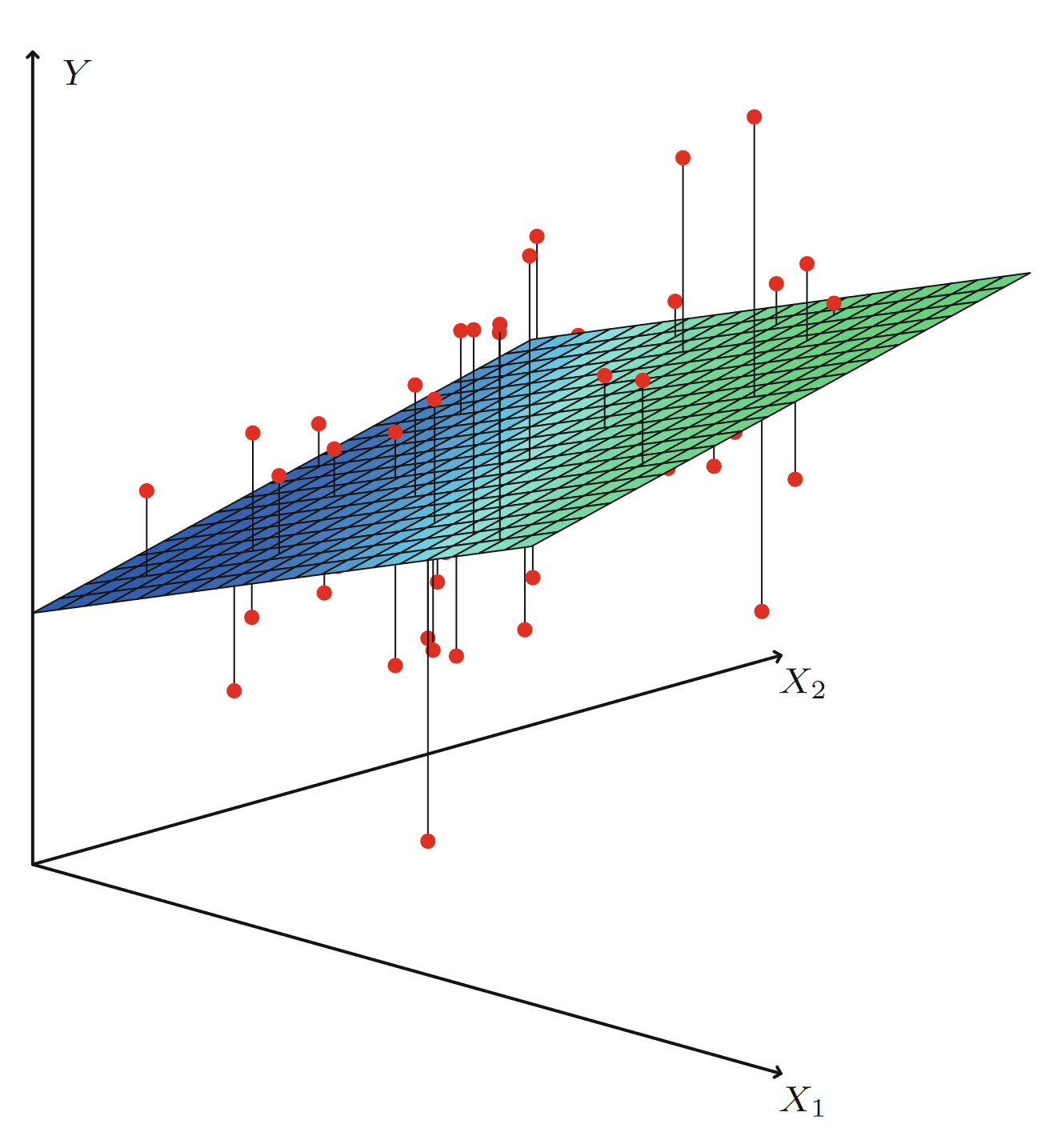
In the real world you often have more than just one feature, we could for example also add height. The idea stays the same, it just becomes a little more difficult to visualize, the errors are now the distance to a hyperplane instead of a line.

Here is a graph on how you might visualize this from one of my favorite ML Books, Introduction to Statistical Learning with R :

Well, this is it. You learned Linear Regression. Linear Regression aims to find a linear model from a set of features ${x}$ that minimizes an error function, which in most cases is the sum of squared errors to the target variable ${y}$.

Linear Models

Simply put a model ${f(x)}$ is linear if the result stays the same, whether you first change the input by adding ${f(a + b) = f(a) + f(b)}$, or scaling ${f(cx) = cf(x)}$, then apply the function. Or if you apply the function and then transform the output by adding ${f(a + b) = f(a) + f(b)}$ or scaling ${f(cx) = cf(x)}$.

Intermediate going further

Todo. :-) Coming soon.